5.3 Scheduling Algorithms
The following subsections will explain several common scheduling strategies, looking at only a single CPU burst each for a small number of processes. Obviously real systems have to deal with a lot more simultaneous processes executing their CPU-I/O burst cycles.
5.3.1 First-Come First-Serve Scheduling, FCFS
- FCFS is very simple - Just a FIFO queue, like customers waiting in line at the bank or the post office or at a copying machine.
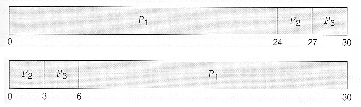
- Unfortunately, however, FCFS can yield some very long average wait times, particularly if the first process to get there takes a long time. For example, consider the following three processes:
Process Burst Time
- In the first Gantt chart below, process P1 arrives first. The average waiting time for the three processes is ( 0 + 24 + 27 ) / 3 = 17.0 ms.
- In the second Gantt chart below, the same three processes have an average wait time of ( 0 + 3 + 6 ) / 3 = 3.0 ms. The total run time for the three bursts is the same, but in the second case two of the three finish much quicker, and the other process is only delayed by a short amount.
- FCFS can also block the system in a busy dynamic system in another way, known as the convoy effect. When one CPU intensive process blocks the CPU, a number of I/O intensive processes can get backed up behind it, leaving the I/O devices idle. When the CPU hog finally relinquishes the CPU, then the I/O processes pass through the CPU quickly, leaving the CPU idle while everyone queues up for I/O, and then the cycle repeats itself when the CPU intensive process gets back to the ready queue.
5.3.2 Shortest-Job-First Scheduling, SJF
- The idea behind the SJF algorithm is to pick the quickest fastest little job that needs to be done, get it out of the way first, and then pick the next smallest fastest job to do next.
- ( Technically this algorithm picks a process based on the next shortest CPU burst, not the overall process time. )
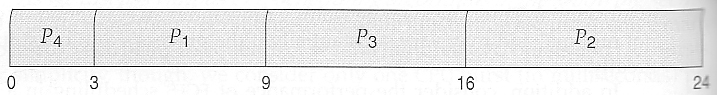
- For example, the Gantt chart below is based upon the following CPU burst times, ( and the assumption that all jobs arrive at the same time. )
Process Burst Time
- In the case above the average wait time is ( 0 + 3 + 9 + 16 ) / 4 = 7.0 ms, ( as opposed to 10.25 ms for FCFS for the same processes. )
- SJF can be proven to be the fastest scheduling algorithm, but it suffers from one important problem: How do you know how long the next CPU burst is going to be?
- For long-term batch jobs this can be done based upon the limits that users set for their jobs when they submit them, which encourages them to set low limits, but risks their having to re-submit the job if they set the limit too low. However that does not work for short-term CPU scheduling on an interactive system.
- Another option would be to statistically measure the run time characteristics of jobs, particularly if the same tasks are run repeatedly and predictably. But once again that really isn't a viable option for short term CPU scheduling in the real world.
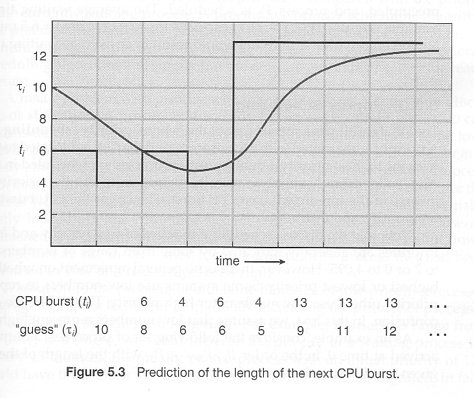
- A more practical approach is to predict the length of the next burst, based on some historical measurement of recent burst times for this process. One simple, fast, and relatively accurate method is the exponential average, which can be defined as follows. ( The book uses tau and t for their variables, but those are hard to distinguish from one another and don't work well in HTML. )
estimate[ i + 1 ] = alpha * burst[ i ] + ( 1.0 - alpha ) * estimate[ i ]
- In this scheme the previous estimate contains the history of all previous times, and alpha serves as a weighting factor for the relative importance of recent data versus past history. If alpha is 1.0, then past history is ignored, and we assume the next burst will be the same length as the last burst. If alpha is 0.0, then all measured burst times are ignored, and we just assume a constant burst time. Most commonly alpha is set at 0.5, as illustrated in Figure 5.3:
- SJF can be either preemptive or non-preemptive. Preemption occurs when a new process arrives in the ready queue that has a predicted burst time shorter than the time remaining in the process whose burst is currently on the CPU. Preemptive SJF is sometimes referred to as shortest remaining time first scheduling.
- For example, the following Gantt chart is based upon the following data:
Process Arrival Time Burst Time
- The average wait time in this case is ( ( 5 - 3 ) + ( 10 - 1 ) + ( 17 - 2 ) ) / 4 = 26 / 4 = 6.5 ms. ( As opposed to 7.75 ms for non-preemptive SJF or 8.75 for FCFS. )
5.3.3 Priority Scheduling
- Priority scheduling is a more general case of SJF, in which each job is assigned a priority and the job with the highest priority gets scheduled first. ( SJF uses the inverse of the next expected burst time as its priority - The smaller the expected burst, the higher the priority. )
- Note that in practice, priorities are implemented using integers within a fixed range, but there is no agreed-upon convention as to whether "high" priorities use large numbers or small numbers. This book uses low number for high priorities, with 0 being the highest possible priority.
- For example, the following Gantt chart is based upon these process burst times and priorities, and yields an average waiting time of 8.2 ms:
Process Burst Time Priority
- Priorities can be assigned either internally or externally. Internal priorities are assigned by the OS using criteria such as average burst time, ratio of CPU to I/O activity, system resource use, and other factors available to the kernel. External priorities are assigned by users, based on the importance of the job, fees paid, politics, etc.
- Priority scheduling can be either preemptive or non-preemptive.
- Priority scheduling can suffer from a major problem known as indefinite blocking, or starvation, in which a low-priority task can wait forever because there are always some other jobs around that have higher priority.
- If this problem is allowed to occur, then processes will either run eventually when the system load lightens ( at say 2:00 a.m. ), or will eventually get lost when the system is shut down or crashes. ( There are rumors of jobs that have been stuck for years. )
- One common solution to this problem is aging, in which priorities of jobs increase the longer they wait. Under this scheme a low-priority job will eventually get its priority raised high enough that it gets run.
5.3.4 Round Robin Scheduling
- Round robin scheduling is similar to FCFS scheduling, except that CPU bursts are assigned with limits called time quantum.
- When a process is given the CPU, a timer is set for whatever value has been set for a time quantum.
- If the process finishes its burst before the time quantum timer expires, then it is swapped out of the CPU just like the normal FCFS algorithm.
- If the timer goes off first, then the process is swapped out of the CPU and moved to the back end of the ready queue.
- The ready queue is maintained as a circular queue, so when all processes have had a turn, then the scheduler gives the first process another turn, and so on.
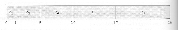
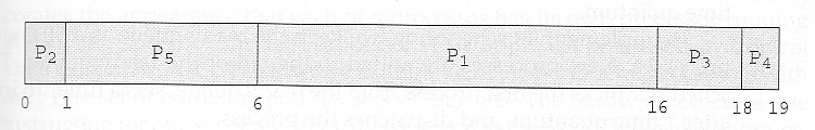
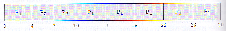
- RR scheduling can give the effect of all processors sharing the CPU equally, although the average wait time can be longer than with other scheduling algorithms. In the following example the average wait time is 5.66 ms.
Process Burst Time
- The performance of RR is sensitive to the time quantum selected. If the quantum is large enough, then RR reduces to the FCFS algorithm; If it is very small, then each process gets 1/nth of the processor time and share the CPU equally.
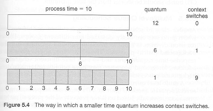
- BUT, a real system invokes overhead for every context switch, and the smaller the time quantum the more context switches there are. ( See Figure 5.4 below. ) Most modern systems use time quantum between 10 and 100 milliseconds, and context switch times on the order of 10 microseconds, so the overhead is small relative to the time quantum.
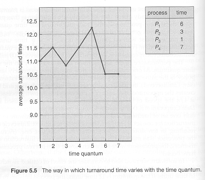
- Turn around time also varies with quantum time, in a non-apparent manner. Consider, for example the processes shown in Figure 5.5:
- In general, turnaround time is minimized if most processes finish their next cpu burst within one time quantum. For example, with three processes of 10 ms bursts each, the average turnaround time for 1 ms quantum is 29, and for 10 ms quantum it reduces to 20. However, if it is made too large, then RR just degenerates to FCFS. A rule of thumb is that 80% of CPU bursts should be smaller than the time quantum.
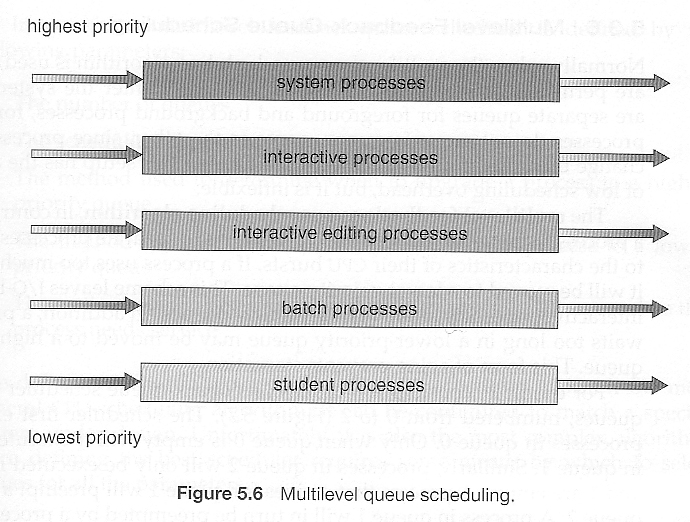
5.3.5 Multilevel Queue Scheduling
- When processes can be readily categorized, then multiple separate queues can be established, each implementing whatever scheduling algorithm is most appropriate for that type of job, and/or with different parametric adjustments.
- Scheduling must also be done between queues, that is scheduling one queue to get time relative to other queues. Two common options are strict priority ( no job in a lower priority queue runs until all higher priority queues are empty ) and round-robin ( each queue gets a time slice in turn, possibly of different sizes. )
- Note that under this algorithm jobs cannot switch from queue to queue - Once they are assigned a queue, that is their queue until they finish.
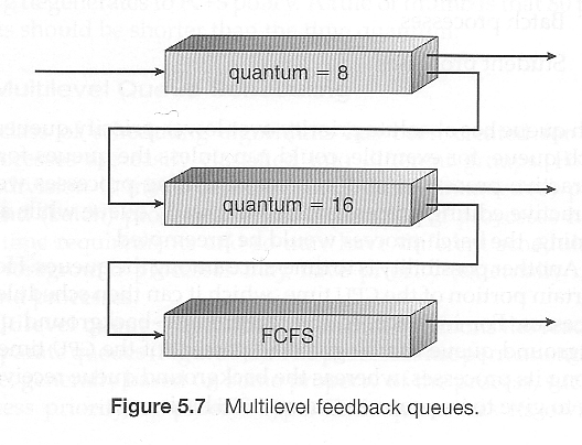
5.3.6 Multilevel Feedback-Queue Scheduling
- Multilevel feedback queue scheduling is similar to the ordinary multilevel queue scheduling described above, except jobs may be moved from one queue to another for a variety of reasons:
- If the characteristics of a job change between CPU-intensive and I/O intensive, then it may be appropriate to switch a job from one queue to another.
- Aging can also be incorporated, so that a job that has waited for a long time can get bumped up into a higher priority queue for a while.
- Multilevel feedback queue scheduling is the most flexible, because it can be tuned for any situation. But it is also the most complex to implement because of all the adjustable parameters. Some of the parameters which define one of these systems include:
- The number of queues.
- The scheduling algorithm for each queue.
- The methods used to upgrade or demote processes from one queue to another. ( Which may be different. )
- The method used to determine which queue a process enters initially.